Atmospheric attraction computation service (Atmacs)

Computation scheme

---

Atmospheric effects on gravity

Routinely, atmospheric density data and surface pressure is provided by DWD for the global ICON model (see Meteorological and ocean models). This data is used as input for the atmospheric loading computation. Attraction and deformation contributions are computed separately: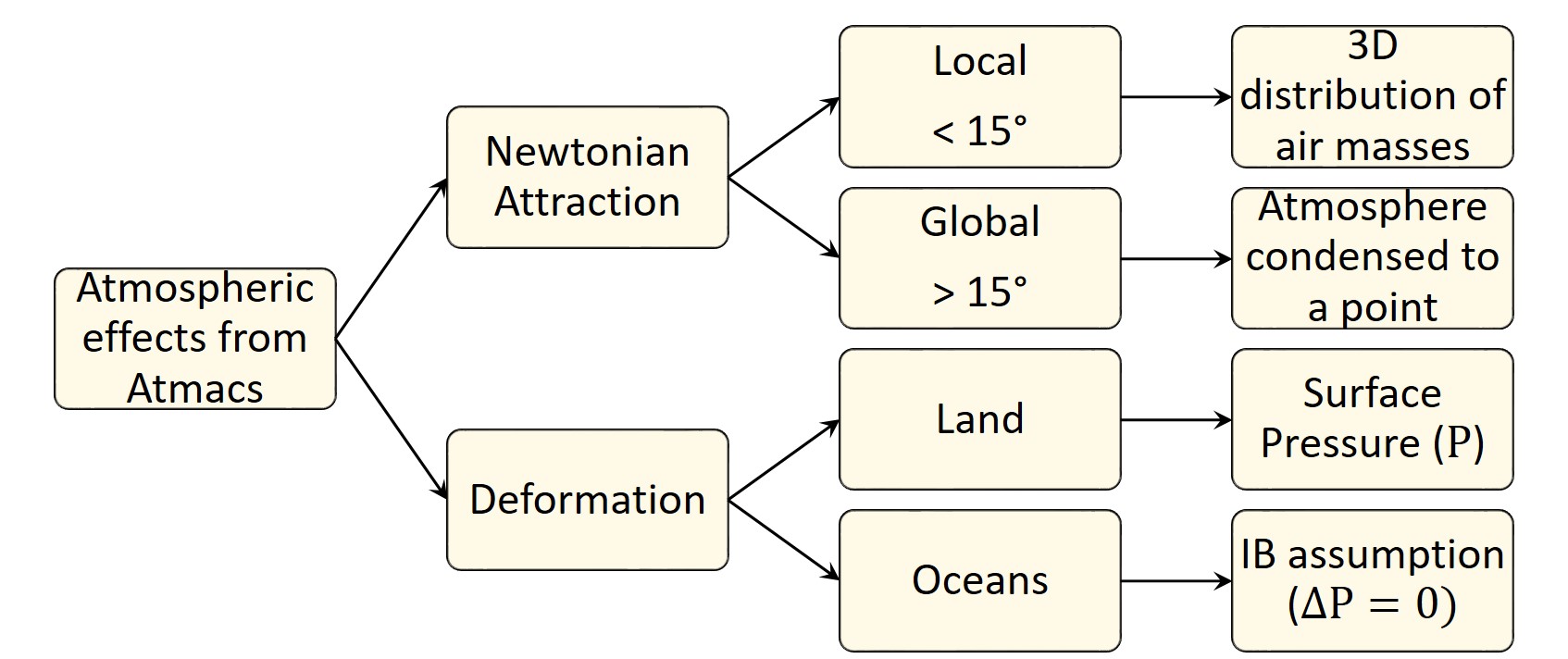

Newtonian attraction

The calculation of Newtonian attraction effects is divided into a region where the vertical air mass distribution is considered and a remaining global part. Despite this distinction, the computation of gravity effects is based on point masses which depends on the geometrical relation between the observation point P and the air mass element Q: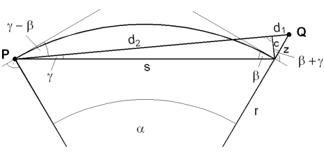

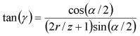
The elevation angle γ and the distance d (d1 + d2) between both points are obtained from the spherical distance α and the height of the cell centre above ground z. Here, the surface topography was used as given in the atmospheric models. From this, γ and d are obtained from:


with r being the radius of a spherical Earth. Using the density and the distance, the point mass attraction of a cell with volume V can be computed according to:

where G is the gravitational constant. The three components of gravitational acceleration in a local coordinate system with x pointing towards east, y towards north and z upwards are derived from trigonometrical relationships:

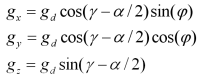
where Phi is the azimuth of the mass point. All contributions are summed up component-wise.

Local (<30°)

Within the local zone, the 3D distribution of mass is considered, where the air density is directly used to infer the mass of the cell. Since point masses are not valid close to the computation point, a further densification of each cell is performed nearby the station. The densification is then applied by linear interpolation, depending on the distance from the computation point. For the recent global ICON model with a spatial resolution of about 13 km, different densifications factors are applied depending on the distance of the cell to the computation point:

Range	Densification factor
Innermost cell	500
Up to 25 km	100
Up to 200 km	20
Up to 30°	1

Global (>30°)

Beyond the limits of the local zone, the mass of each air column is condensed to its centre of mass, located at about 4.5 km height. Although this is a simplification, the big distance allows this approach (see Kluegel and Wziontek 2010). Then the surface pressure P can be easily expressed as a mass by:

with A being the area of the cell and g the standard gravity (9.80665 m/s2).

Deformation

Elastic deformation effects are computed following the classical approach of Farrell (1972), applying load Love numbers from the Preliminary Earth Model (PREM) assuming a Moho depth of 40km as given by Jentzsch (1997). The mass load is derived from surface atmospheric pressure assuming hydrostatic equilibrium. Over the oceans, the IB hypothesis was assumed to be valid, including the static contribution of the atmosphere to ocean-bottom pressure. Practically, atmospheric pressure over oceans is set to a mean pressure value over the ocean area.

To discriminate between continents and oceans, a coastline definition is implemented based on the spatial resolution of the global ICON model and considering large catchments such as the Caspian Sea which behaves as a lake as it is not connected to the global ocean, and the major lakes as the Great Lakes in North America or lakes Victoria and Tanganyika in Africa.

How to improve the temporal resolution

The temporal resolution 3 hours given in the ICON solution can be improved using highly resolved local air pressure data recorded at the station. To do so, a remove-restore technique can be applied: Extract the model air pressure (col 2) from the total atmospheric effect using a constant admittance factor being typical for the local zone (e.g. 2 or 2.5 nm/s2/hPa). Interpolate and re-introduce the air pressure basing on your high-resolution data using the same admittance factor. It could be necessary to vary the admittance factor in order to obtain the best result. In summary,

where:

• g_atm is the final atmospheric correction;
• local_press is the local air pressure record;
• model_press is the air pressure from the model (provided in the Atmacs file);
• local_att is the local attraction as given in Atmacs;
• global_att is the global attraction as given in Atmacs;
• def is the deformation effects as given in Atmacs;
• ocean_int is the ocean interface as given in Atmacs.

---

Non-tidal ocean loading (NTOL) effects

Ocean-bottom pressure anomalies as obtained from the ocean simulation of MPIOM are first resampled on a regular grid of 0.25° x 0.25° spatial resolution. In order to infer mass anomalies (m) from ocean-bottom pressure (P) anomalies, a hydrostatic behaviour is assumed following


with A being the area of the cell and g the standard gravity (9.80665 m/s2).

Newtonian attraction and deformation effects are then computed for each of the stations with the SPOTL software package (Agnew, 2012) using the same Green’s functions used for the atmospheric loading contribution.

---

Computation of previous solutions of Atmacs

In the following, a brief description of the computation of the old solutions of Atmacs is described.

Regional 3D model

According to Newton's law the attraction of each cell is computed from its mass or density and its distance to the observation point. Assuming the atmosphere to be an ideal gas, the density results from:

where p_bot and p_top are the air pressure at the bottom and top of the corresponding layer, R is the gas constant for dry air (287 J/(kg K)) and T_v the virtual temperature. T_v is the equivalent temperature of dry air having the same density as wet air at a specific temperature, and can be computed from the air temperature T and the specific humidity s according to:

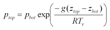
The pressure at the layer top is computed from the bottom pressure and the virtual temperature, which is assumed to be constant throughout the layer:

Local cylinder model

Since the point mass approximation is inadequate in the local zone, the spatial extent of the masses must be taken into account. For a number of cells (usually 9) around the observation point these cells are replaced by a cylinder of the same base area, which is divided into a pile of disks matching the layers of the weather model. The density within each disk is computed from the surface pressure and the virtual temperature of the corresponding layer, analogous to the regional model. The vertical attraction of each disk is computed using the analytical expression:

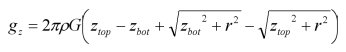
where z_bot and z_top are the heights of the disk's base and top above ground and r is the radius of the disk.